Stock price prediction is the hottest topic now a days. If you can predict stock prices with a reasonable degree of accuracy, you can use that information to make a lot of money in the stock market. This is the dream of the quants. Did you read the Market Wizard book series by Jack Schwager? Quants work all day developing algorithms that they then use to trade in the stock market. Today algorithms are trading against algorithms. Almost 80% of the trades that are being made in Wall Street are being made by algorithms.It is being claimed that the future belongs to algorithmic trading.
Stock market is a dynamic non linear system. Every minute new information is being incorporated into stock prices. Especially if there is breaking company news, it will shoot the stock up or down depending on whether company news is good or bad. Some have tried to model the stock market using Chaos Theory. But I think the key to success lies in building a dynamical model that reevaluates your prediction every minute or five minute in real time.Reading good books on investing and trading can take your trading and investing skills to a higher level.This is the list of 40 books that every investor and trader should read.
Now most of the days are lackluster. There is no surprise. Stocks move as they have been moving countless days before. But then the Black Swan event takes place. This is the event that cannot be predicted at all. Famous Black Swan events are the October 1987 stock market crash or the May Flash Crash of 2010. This is the time when most traders and investors lose most of their portfolios. So predicting the stock market is a difficult game. There are many factors that are at play. Human emotions, company financial statements, overall economic conditions, political situation, consumer confidence etc. There are host of factors that are involved in determining the stock market direction. But there are a breed of analysts known as Quants who get employed by Wall Street firms to predict the stock market. Quants usually have PhDs in maths, physics and finance. They build complicated mathematical models that they use to predict the stock market. But they are not always right. The stock market crash of 2008 has been blamed on quants. Some people think that hedge funds can bring the next global financial meltdown.Read this post on will the hedge funds bring the next global financial meltdown.
Trend trading is what has made fortunes for most traders who ultimately succeeded in this game of stock trading. Trend trading is also known as trend following. In this post we try to predict the stock closing price next day. We can then refine our model and predict stock closing price after say 5 days or even 10 days. Technical analysis is the traditional approach to trend trading. But more and more quantitative methods are being employed in predicting the trend in the market. Read this post on trend following: how millions are made in up or down markets.
In this post we try to build a stock price prediction model that use Support Vector Regression (SVR). SVRs are a statistical and mathematical model that maps the original non linear data into a higher dimensional space in an attempt to make it linear by using a transformation.The most popular transformation is the Radial Basis Function (RBF). If you don’t know anything about SVRs, you should watch this videos below that explains Support Vector Machines (SVMs) in detail. Watching the video will explain many things that you cannot learn by reading.
Now after watching the video you should have a more clear idea on how these Support Vector Machines work. Support Vector Machines are of two types, Support Vector Classification Machines and Support Vector Regression Machines.Classification is when you try to predict the categorical data like Up or Down. Regression is when we want to predict a continuous variable like the temperature or the stock price tomorrow.
In this post we will use a SVRM to predict the next day Apple Stock Price. We will be using R scripting language. R is a powerful open source data analysis and machine learning language. You should have both R and RStudio installed on your computer. First we download the Apple stock AAPL daily data from Yahoo Finance. Below is a plot of the downloaded data.Read this post on the tale of 2 hedge funds-interview with a billionaire mathematician hedge fund manager.
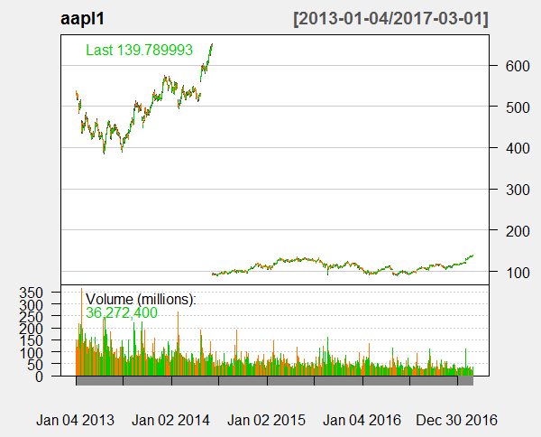
As you can see in the above plot, there is a huge gap. This was caused when Apple stock split took place. As you can see the Apple stock split took place somewhere in June 2014. To be precise the last time Apple stock split took place was on June 9th 2014. The split ratio was 7-1. What this means is that each stock was replaced with 7 stocks. Stock splitting is mostly done to bring the stock price down and make it more accessible to the general public. Pre split Apple stock price was $645 per share. This was quite high for most investors. So Apple company decided to split the stock. As you can see now the Apple stock is trading below $150 per share. So the price has come down and more people can invest in Apple stock. Before 2014, three more times Apple stock had been split. These dates are February 28th, 2005 Apple stock was split 2-1, June 21st, 2000 Apple stock was split 2-1 and June 16th !987, Apple stock was split 2-1 for the first time. Stock market is basically a loser’s game. You need to learn how to become better at losing. Watch this documentary how to win the loser’s game. Below is the plot of the Apple stock AAPL daily candlesticks for the last 3 months.
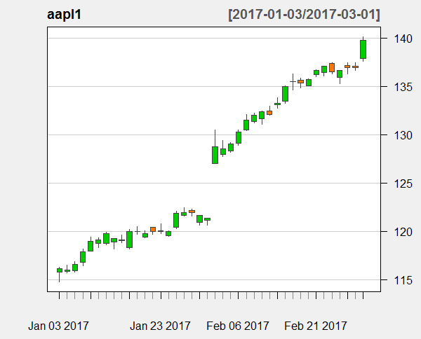
Now once again you can see a big gap in the above AAPL chart. These gap mostly happens when there is some big company news. As you can see there is a strong uptrend in Apple stock. The gap that you can see in AAPL price in the above chart was caused by a renewed optimism about the iPhone. AAPL is once again the darling of Wall Street. All those rumors about the company losing its innovation after Steve Jobs have it seemed come to an end. AAPL is in a strong uptrend once again backed by strong optimism of the investors. So as said above in the start, predicting stock prices can be a tricky thing. You can never be 100% accurate. As you can see just a few positive reviews about the future of iPhone caused AAPL to jump up with a big gap. Below is a simple model that does not take into account news and market sentiment. Most of the time, you will find this model working but on and off you will see the price prediction to be wide off the mark. In the future post I will write on how to incorporate news and market sentiment into out model as well so that we improve our stock price prediction. Read this post on how to start a quant hedge fund.
> #download AAPL Daily and Weekly data from Yahoo Finance
> #load library
> library(quantmod)
Loading required package: xts
Loading required package: zoo

Attaching package: ‘zoo’

The following objects are masked from ‘package:base’:

    as.Date, as.Date.numeric

Loading required package: TTR
Version 0.4-0 included new data defaults. See ?getSymbols.
> #create an environment
> aapl <- new.env()
> #first we download the daily time series data from Yahoo Finance
> getSymbols("AAPL", env = aapl, src = "yahoo",
+            from = as.Date("2013-01-04"), to = as.Date("2017-03-01"))
    As of 0.4-0, ‘getSymbols’ uses env=parent.frame() and
 auto.assign=TRUE by default.

 This  behavior  will be  phased out in 0.5-0  when the call  will
 default to use auto.assign=FALSE. getOption("getSymbols.env") and
 getOptions("getSymbols.auto.assign") are now checked for alternate defaults

 This message is shown once per session and may be disabled by setting
 options("getSymbols.warning4.0"=FALSE). See ?getSymbols for more details.
[1] "AAPL"
>
> aapl1 <- aapl$AAPL
>
> tail(aapl1)
           AAPL.Open AAPL.High AAPL.Low AAPL.Close AAPL.Volume AAPL.Adjusted
2017-02-22    136.43    137.12   136.11     137.11    20745300        137.11
2017-02-23    137.38    137.48   136.30     136.53    20704100        136.53
2017-02-24    135.91    136.66   135.28     136.66    21690900        136.66
2017-02-27    137.14    137.44   136.28     136.93    20196400        136.93
2017-02-28    137.08    137.44   136.70     136.99    23403500        136.99
2017-03-01    137.89    140.15   137.60     139.79    36272400        139.79
> class(aapl1)
[1] "xts" "zoo"
> dim(aapl1)
[1] 1046    6
>
> # Plot the daily price series and volume showing stock split
> chartSeries(aapl1,theme="white")
>
> # Plot the daily price series and volume without showing stock split
> chartSeries(aapl1,theme="white", TA=NULL,  subset='last 3 months')
>
> ######################1 Day Ahead Prediction######################
>
> #using the window operator
> #define lookback
> lb=900
> x <- nrow(aapl1)
> data1 <- aapl1[(1:x), -(5:6)]
> data1 <- data1[,-(1:3)]
> tail(data1)
           AAPL.Close
2017-02-22     137.11
2017-02-23     136.53
2017-02-24     136.66
2017-02-27     136.93
2017-02-28     136.99
2017-03-01     139.79
> dim(data1)
[1] 1046    1
>
> data1$Close_0 <- data1[,1]
> data1$Close_1 <- data1[,1]
> data1$Close_2 <- data1[,1]
>
> data1$Close_0 <- lag(data1$Close_0)
> data1$Close_1 <- lag(data1$Close_0)
> data1$Close_2 <- lag(data1$Close_1)
>
> data1 <- data1[, c(1,4,3,2)]
> tail(data1)
           AAPL.Close Close_2 Close_1 Close_0
2017-02-22     137.11  135.35  135.72  136.70
2017-02-23     136.53  135.72  136.70  137.11
2017-02-24     136.66  136.70  137.11  136.53
2017-02-27     136.93  137.11  136.53  136.66
2017-02-28     136.99  136.53  136.66  136.93
2017-03-01     139.79  136.66  136.93  136.99
>
> data1$Base_Value <- data1$Close_1
> data1 <- data1[, c(1,4,5,2,3)]
> tail(data1)
           AAPL.Close Close_0 Base_Value Close_2 Close_1
2017-02-22     137.11  136.70     135.72  135.35  135.72
2017-02-23     136.53  137.11     136.70  135.72  136.70
2017-02-24     136.66  136.53     137.11  136.70  137.11
2017-02-27     136.93  136.66     136.53  137.11  136.53
2017-02-28     136.99  136.93     136.66  136.53  136.66
2017-03-01     139.79  136.99     136.93  136.66  136.93
>
> data1$Close_0 <- data1$Close_0-data1$Base_Value
> data1$Close_2 <- data1$Close_2-data1$Base_Value
> data1$Close_1 <- data1$Close_1-data1$Base_Value
>
> data1 <- data1[,-5]
> data1 <- data1[,c(2,3,4,1)]
> tail(data1)
             Close_0 Base_Value   Close_2 AAPL.Close
2017-02-22  0.979996     135.72 -0.369995     137.11
2017-02-23  0.410004     136.70 -0.979996     136.53
2017-02-24 -0.580002     137.11 -0.410004     136.66
2017-02-27  0.130005     136.53  0.580002     136.93
2017-02-28  0.269989     136.66 -0.130005     136.99
2017-03-01  0.060012     136.93 -0.269989     139.79
>
> #load the kernlab library
>
> library(kernlab)
>
>
> # train a support vector machine
> filter <- ksvm(AAPL.Close~.,data=data1[1:(x-1),1:4],kernel="rbfdot",
+                kpar=list(sigma=0.05),C=5000,cross=1)

 cross should be >1 no cross-validation done!

>
> print(filter)
Support Vector Machine object of class "ksvm"

SV type: eps-svr  (regression)
 parameter : epsilon = 0.1  cost C = 5000

Gaussian Radial Basis kernel function.
 Hyperparameter : sigma =  0.05

Number of Support Vectors : 32

Objective Function Value : -16860.11
Training error : 0.009879
>
>
> ## predict the next candle
> pred <- predict(filter, data1[x, 1:3])
>
> pred
         [,1]
[1,] 139.7174
You can see above actual AAPL price is $139.79 while our predicted AAPL price is $139.7174 which is quite good. Training error for our model is 0.009 which is very good. We have skipped cross validation as it was taking more time and was not improving price prediction. Now standard economics is not able to explain most of the things that happen in the stock market. I have developed this course Behavior Finance For Traders. In this course on Behavior Finance For Traders, I show you how most of the things that are happening in the stock market are easily explained by this new subject. Going through this course will help you become a better trader and a better investor.